Linear classification

Vivek Yadav, PhD

Overview

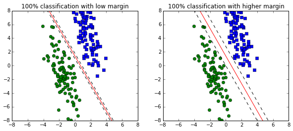
In a previous post, we discussed how a linear classifier can be made using support vector machines. One disadvantage of an SVM is that a classifier with NO regularization cost is updated only until all the training points are classified correctly. SVM based-classifiers do not distinquish models based on how well or confidently they classify the data. As a result it is difficult to compare the quality of two models. A softmax classifier is a better choice when we are also concerned about the quality of classification. For example, both the SVM models presented below classify the data accurately, however, the one on the right is prefered because it has higher margin. A SVM update rule without regularized weight will not be able to pick out this difference. Worse, it is possilbe that with regularized weights the SVM method chooses the classifier with a smaller margin.

import numpy as np
import matplotlib.pyplot as plt
import time 
%matplotlib inline
np.random.seed(2016)

X1 = np.random.randn(100)+1.5
Y1 = -2*(X1)+8+2*np.random.randn(100)
X2 = np.random.randn(100)-1.5
Y2 = -2*(X2)-4 + 2*np.random.randn(100)
X = np.linspace(-8,8,200)
Y = -2*X+2

plt.figure(figsize=(10,4))
plt.subplot(1,2,1)
plt.plot(X1,Y1,'s',X2,Y2,'o')
plt.plot(X,-2*X+1.4,'r',
        X,-2*X+1.8,'--k',
        X,-2*X+1.0,'--k')
plt.ylim(-8,8)
plt.xlim(-8,8)
plt.title('100% classification with low margin')
plt.subplot(1,2,2)
plt.plot(X1,Y1,'s',X2,Y2,'o')
plt.plot(X,-2*X+1.4,'r',
        X,-2*X+2.8,'--k',
        X,-2*X+0,'--k')
plt.ylim(-8,8)
plt.xlim(-8,8)
plt.title('100% classification with higher margin')

Softmax classifier

In a softmax classifier, first a weight matrix $W $ is obtained. This matrix when multiplied by the data $ X $ gives the activations corresponding to each class. We interpret these activations as the log-probabilites of the data point belonging to each class. Therefore, the normalized probability of data belong to individual class is,

$a = W^T X_i$

$P_{j_{class}}( x_i) = \frac{exp(a_{j_{class}}(x_i))}{\sum_{j=1}^{M} exp(a_{j}(x_i))} ,$ where $ P_{j_{class}}( x_i) $ is the probability of the point $ x_i $ belonging to the $ j_{class} $, and $ M $ is the number of classes. The predicted class is then the class with the highest probability.

The Softmax classifier minimizes the cross-entropy between the estimated class probabilities ( $ P_{j_{class}}( x_i) $ ) and the true probability.

$J = \sum_{i=1}^N -log\left( \frac{exp(a_{ic})}{ \sum_{j=1}^M exp(a_{j}) } \right) = \sum_{i=1}^N \left[- a_{ic} + log \left( \sum_{j=1}^M exp(a_{j}) \right) \right]$

where $ ic $ is the label of the correct class and $N $ is the number of training points in the data set.

For linear activations with regularization, the cost function becomes, $J = \sum_{i=1}^N \left[- W_{i_c,}^T X_{i} + log \left( \sum_{j=1}^M exp(W_{j,}^T X_{j}) \right) \right] + \frac{\lambda}{2} || W || ^2$

Derivating of the cost function with respect to W

Note that cost expression above is a scalar, therefore the derivative with respect to a matrix is the matrix of the derivative of the scalar function with each term of the matrix.

Taking derivative with respect to $ W $,

$\frac{ \partial J }{\partial W } = \sum_{i=1}^N \left[- \left( \begin{array}{c} 0_{i_c-1 \times n} \\ X_{i}^T \\ 0_{m-i_c \times n}\\ \end{array} \right) + \frac{1}{\sum_{j=1}^M exp(W_{j,}^T X_{i})} \left( \begin{array}{c} X_{i}^T exp(W_{1,}^T X_{i}) \\ X_{i}^T exp(W_{2,}^T X_{i}) \\ \vdots \\ X_{i}^T exp(W_{m,}^T X_{i})\\ \end{array} \right) \right] + \lambda W$

Rewriting the ratios of exponents as probability, $\frac{ \partial J }{\partial W } = \sum_{i=1}^N X_{i}^T \left[- \left( \begin{array}{c} 0_{i_c-1 \times 1} \\ 1 \\ 0_{m-i_c \times 1}\\ \end{array} \right) + \left( \begin{array}{c} p_1(X_i) \\ p_2(X_i) \\ \vdots \\ p_m(X_i) \\ \end{array} \right) \right] + \lambda W$

We next define a vector $ P_{hat}$ whose terms are equal to the class probabilities for all the incorrect classes, and correct class probability minus 1. $\frac{ \partial J }{\partial W } = \sum_{i=1}^N X_{i}^T P_{hat}(X_i)+ \lambda W$

$\frac{ \partial J }{\partial W } = X^T P_{hat}(X)+ \lambda W$ $\frac{ \partial J }{\partial W } = X^T P_{hat}(X) + \lambda W$

The weight update rule is given by the expression below. Intuitively, this rule tries to move along directions that minimizes the probability of the incorrect classes. Further, subtracting 1 from the correct class probability has the effect of minimizing the probability of incorrectly identifying the correct class.

$W = W - \mu \frac{ \partial J }{\partial W }$

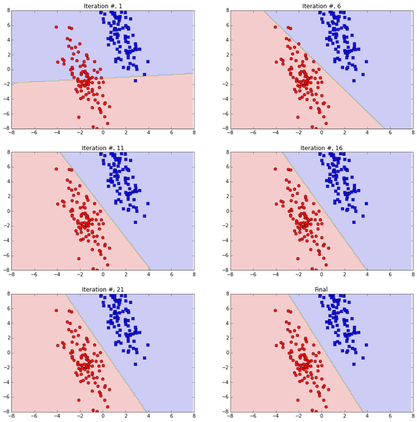
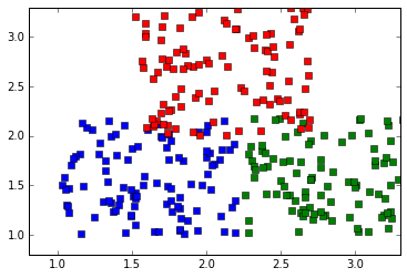
Softmax- 2 class example

Lets revisit the example from before. The task is to find a line that best separates the points below.

def get_loss_grad(X,W,target):
    max_rm = np.max(np.dot(W.T,X))
    pred = np.exp(np.dot(W.T,X)-10)
    sum_probs = np.max(pred,axis=0)
    #pred_grid = np.argmax(np.dot(W.T,X_grid),axis=0)
    #pred_grid_rs = np.reshape(pred_grid,(num_x,num_y))
    scores =(pred/sum_probs)
    J = -np.sum(scores[target,range(len(target))])
    dJdW = scores
    dJdW[target,range(len(target))] -= 1
    dJdW = np.dot(dJdW,X.T).T + lam*W
    return J,dJdW

def plot_classifier():
    plt.contourf(xx, yy, np.asarray(pred_grid_rs), alpha=0.2)
    plt.plot(X1,Y1,'bs',X2,Y2,'ro')
    plt.ylim(-8,8)
    plt.xlim(-8,8)
    
def sfmx_predict(W,X):
    pred = np.argmax(np.dot(W.T,X),axis=0)
    return pred

W = 0.001*np.asmatrix(np.random.random((3,2)))

lam = 10
lr = 0.001
i_plot = 0
x_cord  = np.hstack((X1, X2)).T
y_cord  = np.hstack((Y1, Y2)).T
X_mod = np.vstack((x_cord,y_cord,np.ones(np.shape(x_cord))))
X_mod = np.asmatrix(X_mod)
target = np.hstack((0*np.ones(np.shape(X1)),np.ones(np.shape(X2))))
target = np.asarray(target,dtype = 'Int8')

plot_option = 1
plt.figure(figsize=(15,15))

W = 0.001*np.asmatrix(np.random.random((3,2)))
xx, yy = np.meshgrid(np.arange(-8, 8, 0.1),
                     np.arange(-8, 8, 0.1))

num_x = len(xx) 
num_y = len(yy) 
X_1 = np.reshape(xx,(num_x*num_y,1))
Y_1 = np.reshape(yy,(num_x*num_y,1))
X_grid = np.hstack((X_1,Y_1,np.ones(np.shape(X_1)))).T
pred_grid = 0
J_all = []
for i_loop in range(200):
    #max_rm = np.max(np.dot(W.T,X_mod))
    #pred = np.exp(np.dot(W.T,X_mod)-10)
    #sum_probs = np.max(pred,axis=0)
    pred_grid = sfmx_predict(W,X_grid)
    pred_grid_rs = np.reshape(pred_grid,(num_x,num_y))
    #scores =(pred/sum_probs)
    #J = -np.sum(scores[target,range(len(target))])
    J,dJdW = get_loss_grad(X_mod,W,target)
    J_all.append(J)
    #dJdW = scores
    #dJdW[target,range(len(target))] -= 1
    #dJdW = np.dot(dJdW,X_mod.T).T + lam*W
    W = W-lr*dJdW 
    if ((i_loop%5==0) & (i_loop<25) & (plot_option == 1)):
        #print i_loop
        i_plot +=1
        plt.subplot(3,2,i_plot)
        plot_classifier()
        title_str = 'Iteration #, %d'%(i_loop+1)
        plt.title(title_str)
    #print lr
plt.subplot(3,2,6)
plot_classifier()
title_str = 'Final'
plt.title(title_str)

x1 = 1+1.2*np.random.rand(100)
y1 = 1+1.2*np.random.rand(100)
c1 = 0*np.ones(100)


x2 = 2.25+1.2*np.random.rand(100)
y2 = 1+1.2*np.random.rand(100)
c2 = 1*np.ones(100)

x3 = 1.5+1.2*np.random.rand(100)
y3 = 2+1.3*np.random.rand(100)
c3 = 2*np.ones(100)

train_data = np.asarray([np.hstack((x1,x2,x3)),np.hstack((y1,y2,y3))])
c = np.asarray(np.hstack((c1,c2,c3)))
col_class = ['bs','gs','rs']

plt.plot(x1,y1,col_class[0])
plt.plot(x2,y2,col_class[1])
plt.plot(x3,y3,col_class[2])
plt.ylim(0.8,3.3)
plt.xlim(0.8,3.3)

def plot_classifier2():
    plt.plot(x1,y1,col_class[0])
    plt.plot(x2,y2,col_class[1])
    plt.plot(x3,y3,col_class[2])
    plt.ylim(0.8,3.3)
    plt.xlim(0.8,3.3)
    plt.contourf(xx, yy, np.asarray(pred_grid_rs), alpha=0.2)

W = 0.0001*np.asmatrix(np.random.random((3,3)))
lam = 1
lr = 0.001
i_plot = 0
x_cord  = np.hstack((x1, x2, x3)).T
y_cord  = np.hstack((y1, y2, y3)).T
X_mod = np.vstack((x_cord,y_cord,np.ones(np.shape(x_cord))))
X_mod = np.asmatrix(X_mod)
target = c
target = np.asarray(target,dtype = 'Int8')

plot_option = 1
plt.figure(figsize=(15,15))

xx, yy = np.meshgrid(np.arange(-8, 8, 0.01),
                     np.arange(-8, 8, 0.01))

num_x = len(xx) 
num_y = len(yy) 
X_1 = np.reshape(xx,(num_x*num_y,1))
Y_1 = np.reshape(yy,(num_x*num_y,1))
X_grid = np.hstack((X_1,Y_1,np.ones(np.shape(X_1)))).T
pred_grid = 0
J_all = []
for i_loop in range(1000):
    
    max_rm = np.max(np.dot(W.T,X_mod))
    pred = np.exp(np.dot(W.T,X_mod)-10)
    sum_probs = np.max(pred,axis=0)
    pred_grid = sfmx_predict(W,X_grid)
    pred_grid_rs = np.reshape(pred_grid,(num_x,num_y))
    scores =(pred/sum_probs)
    J = -np.sum(scores[target,range(len(target))])
    #J,dJdW = get_loss_grad(X_mod,W,target)
    J_all.append(J)
    dJdW = scores
    dJdW[target,range(len(target))] -= 1
    dJdW = np.dot(dJdW,X_mod.T).T + lam*W
    
    
    #pred_grid = sfmx_predict(W,X_grid)
    #pred_grid_rs = np.reshape(pred_grid,(num_x,num_y))
    #J,dJdW = get_loss_grad(X_mod,W,target)
    #J_all.append(J)
    W = W-lr*dJdW 
    if ((i_loop%5==0) & (i_loop<25) & (plot_option == 1)):
        i_plot +=1
        plt.subplot(3,2,i_plot)
        plot_classifier2()
        title_str = 'Iteration #, %d'%(i_loop+1)
        plt.title(title_str)
plt.subplot(3,2,6)
plot_classifier2()
title_str = 'Final'
plt.title(title_str)

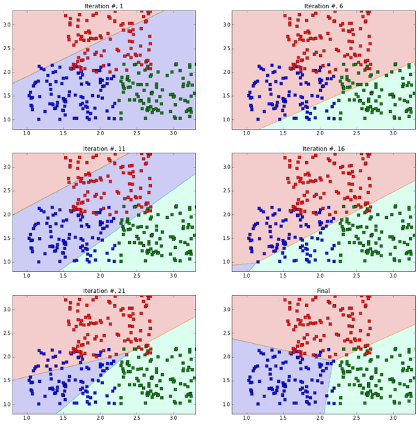
Conclusion

In this post, we developed equations for a softmax classifier and applied it for classification of binary and multi-class problems. I personally prefer the softmax classifier because the class scores have intuitive meaning. Further, the derivative of the loss function is intuitive. The weight update scheme minimizes the probability of incorrect classes and the probability of guessing the correct class wongly.