Linear classification - Support vector machines.
Vivek Yadav, PhD
Overview
In this post, we will go over a linear classification method called Support Vector Machine (SVM). SVM is a discriminative classifier formally defined by a separating hyperplane. In other words, given a labeled set of training data, SVM tries to find a hyperplane that maximizes the distance to points in either class from the plane. We will first define a cost-function, derive the update rule using gradient descent, and test classification performance for various parameters.
import numpy as np
import matplotlib.pyplot as plt
import time
%pylab inline

numpy.random.seed(2016)

X1 = np.random.randn(100)+1.5
Y1 = -2*(X1)+8+2*np.random.randn(100)
X2 = np.random.randn(100)-1.5
Y2 = -2*(X2)-4 + 2*np.random.randn(100)

plt.plot(X1,Y1,'s',X2,Y2,'o')
plt.ylim(-8,8)
plt.xlim(-8,8)
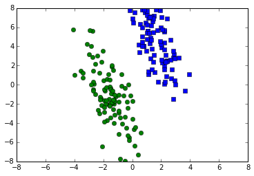
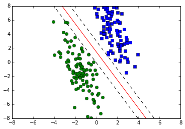
In the example above, we wish to find a line that best separates the two classes. However, there are many lines that can separate the points shown above. For example, in the figure below, all the 3 lines separate the points to the same level. However, intuitively, the blue line appears to be a better choice.
The blue line is suited because it has the greatest distance from the training set in both the classes. Therefore, the blue line is more robust to variations in the data.
X = np.linspace(-8,8,200)
Y = -2*X+2
plt.plot(X1,Y1,'s',X2,Y2,'o')
plt.plot(X,-2*X+2,'b',
         X,-6*X+2,'r',
        X,-1.5*X+2,'m')
plt.ylim(-8,8)
plt.xlim(-8,8)

We wish to find \(W\) and \(b\) such that,
.
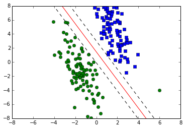
This is also represented by the 3 lines shown below. The red line indicates the best separating line, while the dotted black lines indicate the margin boundaries. To account for cases where the separation is not as clean as that shown below, a slack variable \( \psi \) is introduced.
X = np.linspace(-8,8,200)
Y = -2*X+2
plt.plot(X1,Y1,'s',X2,Y2,'o')
plt.plot(X,-2*X+1.45,'r',
        X,-2*X+3,'--k',
        X,-2*X-.1,'--k')
plt.ylim(-8,8)
plt.xlim(-8,8)
Margin
We define margin as the perpendicular distance between the two black dotted lines. These lines indicate separation between the two black dashed lines. From coordinate geometry, the distance between the two lines \( W^T X = b_1 \) and \( W^T X = b_2 \) is given by \( (b_1 - b_2)/ W \), therefore the margin is
| $$ margin = \frac{2}{ | W | } $$. |
| Maximizing margin is equivalent to minimizing \( | W | \), with the constraint that the points are separated, i.e. |
for each \( i \in \) training data.
This constraint is however a hard constraint, and it is usually desirable to have a soft constraint, where a few points are allowed to be misclassified. In the example below, the green point to the right of the red line looks to be an outlier, therefore, it is acceptable to ignore this point in designing the SVM classifier.
X = np.linspace(-8,8,200)
Y = -2*X+2
plt.plot(X1,Y1,'s',X2,Y2,'o')
plt.plot(6.,-4.,'go')

plt.plot(X,-2*X+1.45,'r',
        X,-2*X+3,'--k',
        X,-2*X-.1,'--k')
plt.ylim(-8,8)
plt.xlim(-8,8)
SVM with soft margins
To allow for misclassifications, a soft margin \( \xi \) is introduced, where \( \xi_i \geq 0 \) is a slack variable that quantifies deviation from the margin lines. If \( \xi_i <1 \), the point is within the two black dashed lines, i.e. within the margin. If \( \xi_i \geq 1 \), then the point is misclassified.
The cost function now becomes,
| Here, \( | W | ^2 \) is the sum of squares of each element in \( W \). |
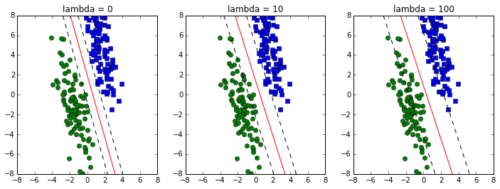
C is a regularization parameter: - small C allows constraints to be easily ignored i.e. large margin - large C makes constraints hard to ignore i.e. narrow margin - \( C = \infty\) enforces all constraints: hard margin
The cost-function above can be rewritten as,
The condition above assures that \( \xi_i \geq 0 \). The right side term above is also refered as hinge-loss. Further, rewriting the above equation using the \( \delta \) notation,
Absorbing the constant term into the vector \(x \) by appending 1 to it, the cost-function above can be rewritten as,
where \( \delta_i = 0 \) if \(i^{th} \) point is classified correctly, else \( \delta_i = 1 \), and \( \lambda = 2/C \).
\(\lambda \) is the new regularization parameter: - large \(\lambda \) allows constraints to be easily ignored i.e. large margin - small \(\lambda \) makes constraints hard to ignore i.e. narrow margin - \(\lambda = 0 \) enforces all constraints: hard margin
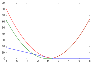
The cost function above can be differentiated with respect to \( W \) to obtain solution that classifies the data while maximizing the margin. Note that the cost function has a unique minimum because it is formed by adding a quadratic-convex function to a non-negative monotonous function \( \delta^T \left( 1 - t_i W^Tx_i \right) \).
W = np.linspace(-8,8,200)
fW1 = -2*X+2
fW1 = (np.abs(Y)+Y)/2
plt.plot(W,fW1,'b')
plt.plot(W,W**2,'g')
plt.plot(W,fW1+W**2,'r')
Calculaing derivative
Using the matrix derivatives derived in a previous post, the matrix differentials can be written as,
def plot_fig(W):
    plt.plot(X1,Y1,'s',X2,Y2,'o')
    plt.plot(X,(-W[0]*X-W[2])/W[1])
    plt.plot(X,(-W[0]*X-W[2]+1)/W[1],'k--')
    plt.plot(X,(-W[0]*X-W[2]-1)/W[1],'k--')
    plt.ylim(-8,8)
    plt.xlim(-8,8)


def svm_weights(X_mod,target,W,
                lam,lr,plot_option):
    i_plot = 0
    for i_loop in np.arange(0,1000):
        pred_fun  = np.dot(X_mod,W)
        pred_fun[pred_fun>=1] = 1
        pred_fun[pred_fun<=-1] = -1
        delta_index = [i for i in np.arange(0,len(target)) if target[i] == pred_fun[i]]
        delta= np.ones(np.shape(target))
        delta[delta_index]= 0
        W_mis = np.dot(np.multiply(delta,target),X_mod)
        djdW = np.multiply(lam,W) - W_mis
        W += -lr*djdW
    return W
W = [0,0.1,0]
lam = .1
lr = 0.0005
i_plot = 0
x_cord = np.hstack((X1, X2)).T
y_cord = np.hstack((Y1, Y2)).T
X_mod = np.vstack((x_cord,y_cord,np.ones(np.shape(x_cord)))).T
target = np.hstack((np.ones(np.shape(X1)),-np.ones(np.shape(X2))))
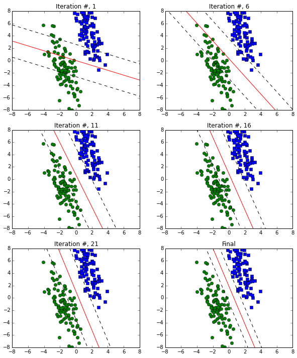
plt.figure(figsize = (10,12))
plot_option = 1
for i_loop in np.arange(0,1000):
# Predict function
pred_fun = np.dot(X_mod,W)
pred_fun[pred_fun>=1] = 1
pred_fun[pred_fun<=-1] = -1
# delta function
delta_index = [i for i in np.arange(0,len(target)) if target[i] == pred_fun[i]]
delta= np.ones(np.shape(target))
delta[delta_index]= 0
# dJdW for misclassified points
dJdW_mis = np.dot(np.multiply(delta,target),X_mod)
# This is second term of the derivative, due to misclassification
djdW = np.multiply(lam,W) - dJdW_mis
W += -lr*djdW
if ((i_loop%5==0) & (i_loop<25) & (plot_option == 1)):
#print i_loop
i_plot +=1
plt.subplot(3,2,i_plot)
plot_fig(W)
title_str = 'Iteration #, %d'%(i_loop+1)
plt.title(title_str)
#W += -lr*djdW
plt.subplot(3,2,6)
plot_fig(W)
plt.title('Final')
Next we will investigate the effect of the parameter \( \lambda \)
plt.figure(figsize=(12,4))
W = [0,0.1,0]
W = svm_weights(X_mod,target,W,
                0.0,lr,plot_option)
plt.subplot(1,3,1)
plot_fig(W)
plt.title('lambda = 0')
W = [0,0.1,0]
W = svm_weights(X_mod,target,W,
                10.0,lr,plot_option)
plt.subplot(1,3,2)
plot_fig(W)
plt.title('lambda = 10')
W = [0,0.1,0]
W = svm_weights(X_mod,target,W,
                100.0,lr,plot_option)
plt.subplot(1,3,3)
plot_fig(W)
plt.title('lambda = 100')
Conclusion
In this post, we saw how support vector machines can be applied to develop a simple 2-class classifier. The same scheme can be extended to multi-class classifiers. We defined a cost-function, parametrized in terms of the support vectors \(W \) that maximized the margin of error while keeping the classification accuracy high. The cost-function had a \( \lambda \) parameter that weighed the margin or error with classification accuracy. Larger \( \lambda \) gave a classifier that would allow more classification errors. Simple gradient descent algorithm was applied to calculate the optimal set of weights. During training, first the support vectors align along the appropriate line, and then the margins become tigher.
One limitation of SVMs is that once the data is classified correctly, the weights do not change because the contribution of the correctly classified error terms is 0. This is especially true for the case were \( \lambda = 0 \). In contrast, a softmax cost function takes into account how well the points are classified and always seeks a better solution.