Instance based learning (Kernel Methods) - Part 2
Vivek Yadav, PhD
1. Motivation
In the previous post I presented one of the simplest instance based machine algorithm, the K-nearest neighbor algorithm (KNN). KNN algorithms make predictions based on k-nearest neighbors alone, and are susceptible to noise in the data. Another short coming is that KNN methods do not consider all the data points in the data set to make predictions. For example, if a given data set is distributed in such a way that there are more points in one region of the input space than another region. In such cases, using the same value of K in different places can lead to noisy and erroneous predictions. In such cases, a good algorithm should use information from more points when making predictions in region with more input points, and use information from fewer points for making prediction in regions that have less data points. Kernel based methods are well suited for such applications. Kernel based methods consider all the data points in the training data set to make predictions. In kernel based methods, first a distance based metric and a weighing function is defined. The predictions for new values are made as weighted average of all the points in the data set, where the weights are calculated individually for every data element for which we wish to make predictions. As all the predictions depend on the weighing function, which in turn depends on the distance metric, it is important to choose these them correctly. In this post, I will present kernel based method for classification and regression.
2. Kernel Regression
First I will present Kernel method for regression, consider the data set shown below.
import numpy as np
import matplotlib
from mpl_toolkits.mplot3d import Axes3D

import matplotlib.cm as cm
import matplotlib.mlab as mlab
import matplotlib.pyplot as plt
% pylab inline
x1 = np.linspace(2,3,10)
x2 = np.linspace(0,8,20)

x = np.hstack((x1,x2))
print np.shape(x)
y = 2*x+6*(np.random.random(np.shape(x))-.5)
plt.plot(x,y,'rs')
Populating the interactive namespace from numpy and matplotlib
(30,)
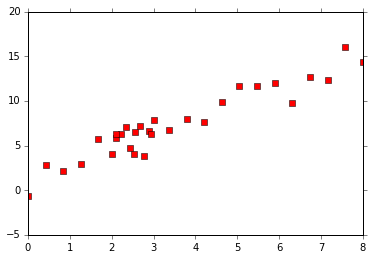
In the example above, it is desirable to use more points to make predictions between the regions 2 and 3, and fewer points for regions beyond 2 and 3. A simple trick to incorporate this information is to use a weighing function whose weight decays as a function of distance. Therefore, the weight function corresponding to the training data point $X_i$ at a point $X$ is given as,
where $d(X,X_i)$ is an appropriate distance function. For our example, $d$ is euclidian distance between X and X_i. $\sigma$ is a parameter that determines how the influence of a point fades. If $\sigma \rightarrow \infty$, then all points have similar importance, and each point in the training data set influences predictions equally. $\sigma \rightarrow 0$, then the influence of each training point is felt at the training point only.
The value for a new point $X$ is given by
3. Weighing function, effect of $\sigma$
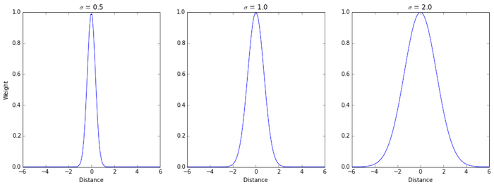
Plots below present how varying the parameter $\sigma$ influences the weighing function. For smaller $\sigma$, the weight decays faster with the distance, whereas for a larger $\sigma$, the weights decay slower. The sigma parameter determines how much influence each point in the data set will have over predictions.
X_x = np.linspace(-6,6,100)

plt.figure(figsize=(15,5))
plt.subplot(1,3,1)
plt.plot(X_x,exp( - X_x**2/.5**2))
plt.title('$\sigma$ = 0.5')
plt.ylabel('Weight')
plt.xlabel('Distance')

plt.subplot(1,3,2)
plt.plot(X_x,exp( - X_x**2/1**2))
plt.title('$\sigma$ = 1.0')
#plt.ylabel('Weight')
plt.xlabel('Distance')

plt.subplot(1,3,3)
plt.plot(X_x,exp( - X_x**2/2**2))
plt.title('$\sigma$ = 2.0')
#plt.ylabel('Weight')
plt.xlabel('Distance')
## Function for kernel regression
def ret_kernel_reg(x_new,x,y,sig):
    W_all = exp( - (x-x_new)**2/sig**2)
    y_pred = np.dot(W_all,y)/np.sum(W_all)
    return y_pred
X_pred_all = np.linspace(0,8.,50)


plt.figure(figsize=(15,15))
plt.subplot(2,2,1)
y_pred_all = [ret_kernel_reg(X_pred_all[i],x,y,.2) for i in np.arange(0,len(X_pred_all))]
plt.plot(x,y,'rs',X_pred_all,y_pred_all,X_pred_all,2*X_pred_all,'--')
plt.title('$\sigma$ = 0.2')
plt.ylabel('Y')
plt.xlabel('X')

plt.subplot(2,2,2)
y_pred_all = [ret_kernel_reg(X_pred_all[i],x,y,1) for i in np.arange(0,len(X_pred_all))]
plt.plot(x,y,'rs',X_pred_all,y_pred_all,X_pred_all,2*X_pred_all,'--')
plt.title('$\sigma$ = 1.0')
plt.ylabel('Y')
plt.xlabel('X')

plt.subplot(2,2,3)
y_pred_all = [ret_kernel_reg(X_pred_all[i],x,y,4.) for i in np.arange(0,len(X_pred_all))]
plt.plot(x,y,'rs',X_pred_all,y_pred_all,X_pred_all,2*X_pred_all,'--')
plt.title('$\sigma$ = 4.0')
plt.ylabel('Y')
plt.xlabel('X')
plt.subplot(2,2,4)
y_pred_all = [ret_kernel_reg(X_pred_all[i],x,y,40.) for i in np.arange(0,len(X_pred_all))]
plt.plot(x,y,'rs',X_pred_all,y_pred_all,X_pred_all,2*X_pred_all,'--')
plt.title('$\sigma$ = 20.0')
plt.ylabel('Y')
plt.xlabel('X')
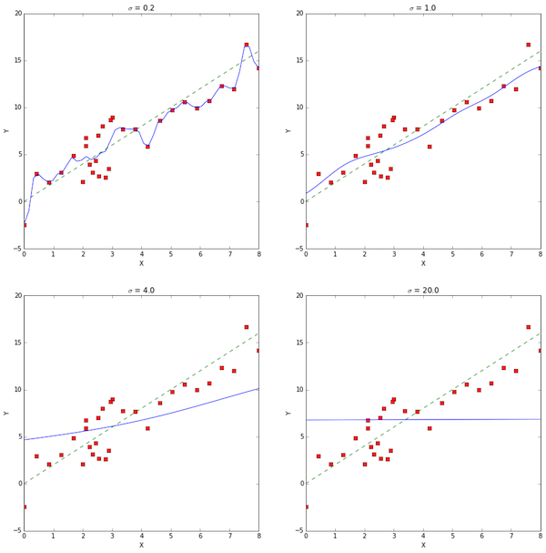
The $\sigma$ parameter in kernel regression weights the influence of each point in the training data set on prediction for a new point. The prediction lines in blue above show that a large $\sigma$ is associated with high bias and low variance, while low $\sigma$ results in an algorithm that is very sensitive to the training data set.
3. Weighing function, effect of $d$
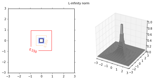
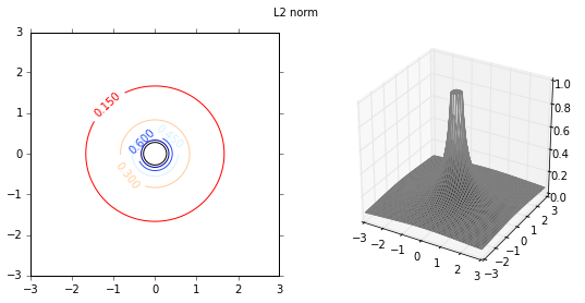
Next I will investigate the effect of various distance functions. I will test 3 specific distance functions, the $L_1$-norm, $L_2$-norm and $L_\infty$-norm. These distance measures are more relevant in a multi-dimensional case, and therfore I will test them on a 2-dimensional data set. First I plot the distance functions.
def plot_fig_countour_dist(X,Y,Z,title_str):
    fig = plt.figure(figsize=(9,4))
    plt.subplot(1,2,1)
    CS = plt.contour(X, Y, Z)
    plt.clabel(CS, inline=1, fontsize=10)
    plt.suptitle(title_str)
    ax = fig.add_subplot(122, projection='3d')
    ax.plot_surface(X,Y,Z,cmap='gray',edgecolors=[.5,.5,.5 ])
plt.figure(figsize = (15,15))
x = np.arange(-3.0, 3.0, .01)
y = np.arange(-3.0, 3.0, .01)
X, Y = np.meshgrid(x, y)
Z1 = (np.abs(X)+np.abs(Y))**-1
Z2 = np.sqrt(X**2+Y**2)**-1
Z_inf = .01*np.maximum(np.abs(X),np.abs(Y))**-1
sig = 1.
Z_gauss = exp( - ((X)**2+Y**2)/sig**2)
Z = np.minimum(14*Z_inf,1)
plot_fig_countour_dist(X,Y,Z,'L-infinity norm')
Z = np.minimum(Z1/4.,1)
plot_fig_countour_dist(X,Y,Z,'L1 norm')
Z = np.minimum(Z2/4.,1)
plot_fig_countour_dist(X,Y,Z,'L2 norm')
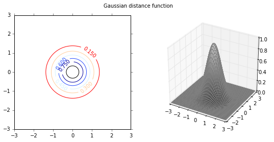
Z = Z_gauss
plot_fig_countour_dist(X,Y,Z,'Gaussian distance function')

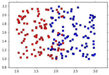
Classification
I will illustrate the effect of distance functions using the example of a 2-class classification. The first 3 weight functions are given as inverse of $L_1$, $L_2$ and $L_{\infty}$ norms, and the last distance function is the gaussian distance function. As the distance function in the first 3 cases is the inverse of various norms, the distance values can be very large depending on the proximity to the training data set. Therefore, the maximum values are capped at 1. The class of new incoming data is given by,
For a 2 class problem, it is assumed that the class labels are -1 and 1, therefor, the class of new incoming data is given by,
def get_dist_fun(X_tr,Y_tr,x_new,y_new,cost_type):
    #
    if cost_type == 1:
        Z1 = (np.abs(X_tr-x_new)+np.abs(Y_tr-y_new))**-1
        Z = np.minimum(Z1/4.,1)
    if cost_type == 2:
        Z2 = np.sqrt((X_tr-x_new)**2+(Y_tr-y_new)**2)**-1
        Z = np.minimum(Z2/4.,1)
    if cost_type == 3:
        Z_inf = .01*np.maximum(np.abs(X_tr-x_new),np.abs(Y_tr-y_new))**-1
        Z = np.minimum(14*Z_inf,1)
    if cost_type == 4:
        sig = 1.
        Z_gauss = exp( - ((X_tr-x_new)**2+(Y_tr-y_new)**2)/sig**2)
        Z = Z_gauss
    return Z

def get_class_kernel(train_data,c,x_new,y_new,cost_type):
    dist_fun = get_dist_fun(train_data[0],train_data[1],x_new,y_new,cost_type)
    ret_class = np.sign(np.dot(dist_fun,c))
    return ret_class
x1 = 1+1.2*np.random.rand(100)
y1 = 1+1.2*np.random.rand(100)
c1 = -1*np.ones(100)


x2 = 1.8+1.2*np.random.rand(100)
y2 = 1+1.2*np.random.rand(100)
c2 = 1*np.ones(100)


train_data = np.asarray([np.hstack((x1,x2)),np.hstack((y1,y2))])
c = np.asarray(np.hstack((c1,c2)))
col_class = ['rs','bs']

plt.plot(x1,y1,col_class[0])
plt.plot(x2,y2,col_class[1])
plt.ylim(0.8,2.3)
plt.xlim(0.8,3.3)
# Plotting decision regions
x_min, x_max = train_data[0,:].min() - 1, train_data[ 0,:].max() + 1.1
y_min, y_max = train_data[1,:].min() - 1, train_data[ 1,:].max() + 1.1


xx, yy = np.meshgrid(np.arange(x_min, x_max, 0.05),
                     np.arange(y_min, y_max, 0.05))
# Distance type 1.
class_test1 = np.zeros(np.shape(xx))
class_test2 = np.zeros(np.shape(xx))
class_test3 = np.zeros(np.shape(xx))
class_test4 = np.zeros(np.shape(xx))
for i in np.arange(0,xx.shape[0]):
    for j in np.arange(0,xx.shape[1]):
        class_test1[i,j] = get_class_kernel(train_data,c,xx[i,j],yy[i,j],1)
        class_test2[i,j] = get_class_kernel(train_data,c,xx[i,j],yy[i,j],2)
        class_test3[i,j] = get_class_kernel(train_data,c,xx[i,j],yy[i,j],3)
        class_test4[i,j] = get_class_kernel(train_data,c,xx[i,j],yy[i,j],4)


plt.figure(figsize=(8,8))
plt.subplot(2,2,1)
plt.contourf(xx, yy, class_test1, alpha=0.4,c = c)
plt.plot(x1,y1,'rs',alpha = 0.5)
plt.plot(x2,y2,'bs',alpha = 0.5)
plt.ylim(0.8,2.3)
plt.xlim(0.8,3.3)
plt.title('L1 norm')

plt.subplot(2,2,2)
plt.contourf(xx, yy, class_test2, alpha=0.4,c = c)
plt.plot(x1,y1,'rs',alpha = 0.5)
plt.plot(x2,y2,'bs',alpha = 0.5)
plt.ylim(0.8,2.3)
plt.xlim(0.8,3.3)
plt.title('L2 norm')

plt.subplot(2,2,3)
plt.contourf(xx, yy, class_test3, alpha=0.4,c = c)
plt.plot(x1,y1,'rs',alpha = 0.5)
plt.plot(x2,y2,'bs',alpha = 0.5)
plt.ylim(0.8,2.3)
plt.xlim(0.8,3.3)
plt.title('L-infinity norm')

plt.subplot(2,2,4)
plt.contourf(xx, yy, class_test4, alpha=0.4,c = c)
plt.plot(x1,y1,'rs',alpha = 0.5)
plt.plot(x2,y2,'bs',alpha = 0.5)
plt.ylim(0.8,2.3)
plt.xlim(0.8,3.3)
plt.title('Gaussian distance function')
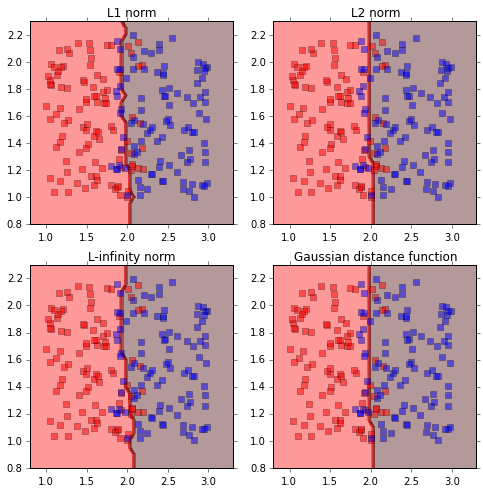
Conclusion
In this post, I present examples of kernel based methods for regression and classificiation. Unlike k-nearest neighbor algorithm, kernel based schemes consider all the data points in the training set. However, the relative importance or weighing of each training point is determined by a distance function. Simulation experiments with using different type of distance function shows that a Gaussian kernel gave smoother decision boundaries, when compared to $L_1$, $L_2$ or $L_{\infty}$ norms. Among $L_1$, $L_2$ or $L_{\infty}$ norms, $L_2$ is better suited because it gives smoother decision boundaries.