Building a student intervention system - EDA
In this post I conduct exploratory data analysis (EDA) on behavioral and demographic data collected in students from two schools. The data can be downloaded from http://tinyurl.com/h2wvk2r.
The data is composed of the following fields,
- ‘school’ student’s school (binary: “GP” or “MS”)
- ‘sex’ student’s sex (binary: “F” - female or “M” - male)
- ‘age’ student’s age (numeric: from 15 to 22)
- ‘address’ student’s home address type (binary: “U” - urban or “R” - rural)
- ‘famsize’ family size (binary: “LE3” - less or equal to 3 or “GT3” - greater than 3)
- ‘Pstatus’ parent’s cohabitation status (binary: “T” - living together or “A” - apart)
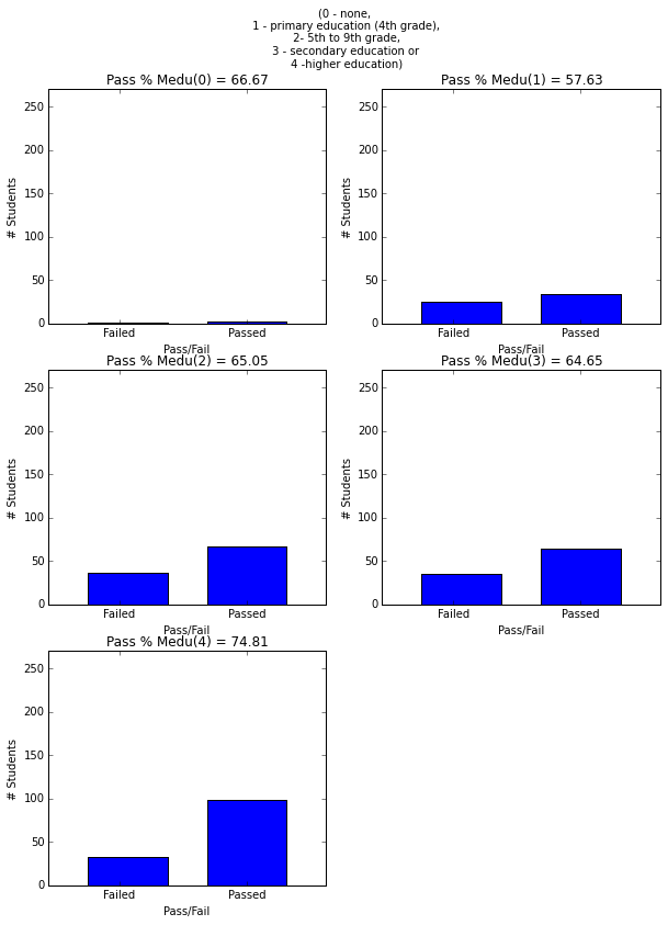
- ‘Medu’ mother’s education (numeric: 0 - none, 1 - primary education (4th grade), 2 - 5th to 9th grade,3- secondary education or 4 - higher education
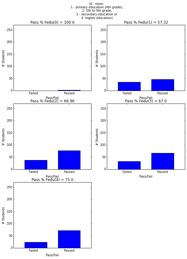
- ‘Fedu’ father’s education (numeric: 0 - none, 1 - primary education (4th grade), 2 - 5th to 9th grade, 3 - secondary education or 4 - higher education
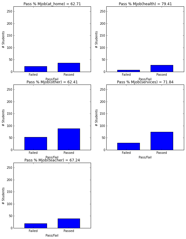
- ‘Mjob’ mother’s job (nominal: “teacher”, “health” care related, civil “services” (e.g. administrative or police), “at_home” or “other”)
- ‘Fjob’ father’s job (nominal: “teacher”, “health” care related, civil “services” (e.g. administrative or police), “at_home” or “other”)
- ‘reason’ reason to choose this school (nominal: close to “home”, school “reputation”, “course” preference or “other”)
- ‘guardian’ student’s guardian (nominal: “mother”, “father” or “other”)
- ‘traveltime’ home to school travel time (numeric: 1 - $<15$ min., 2 - 15 to 30 min., 3 - 30 min. to 1 hour, or 4 - $>1$ hour)
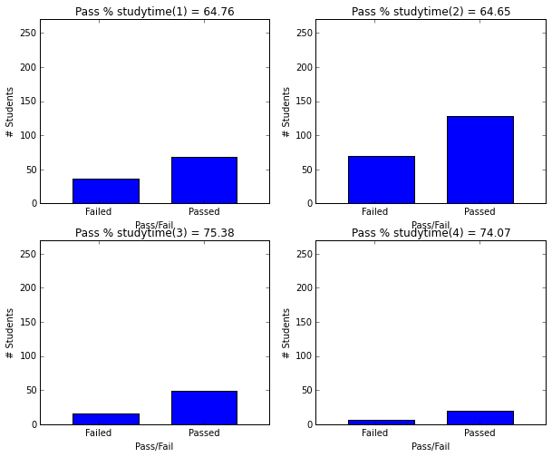
- ‘studytime’ weekly study time (numeric: 1 - $<2$ hours, 2 - 2 to 5 hours, 3 - 5 to 10 hours, or 4 - $>10$ hours)
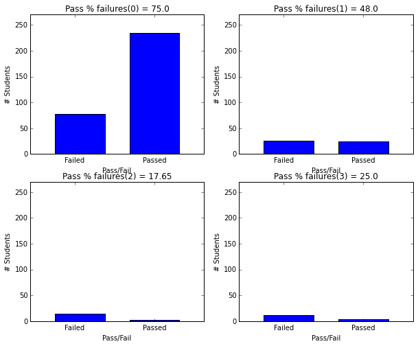
- ‘failures’ number of past class failures (numeric: n if $1<=n<3$, else 4)
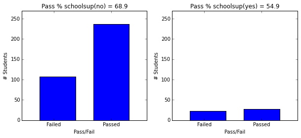
- ‘schoolsup’ extra educational support (binary: yes or no)
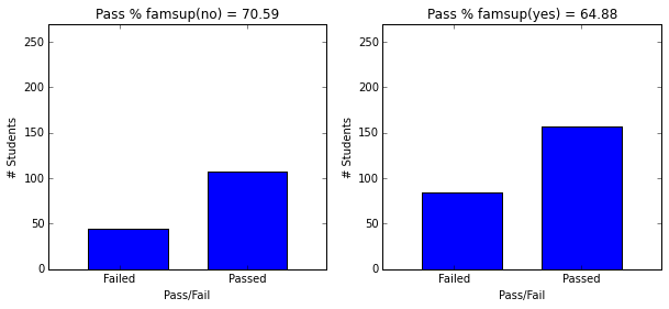
- ‘famsup’ family educational support (binary: yes or no)
- ‘paid’ extra paid classes within the course subject (Math or Portuguese) (binary: yes or no)
- ‘Activities’ extra-curricular activities (binary: yes or no)
- ‘nursery’ attended nursery school (binary: yes or no)
- ‘higher’ wants to take higher education (binary: yes or no)
- ‘internet’ Internet access at home (binary: yes or no)
- ‘romantic’ with a romantic relationship (binary: yes or no)
- ‘famrel’ quality of family relationships (numeric: from 1 - very bad to 5 - excellent)
- ‘freetime’ free time after school (numeric: from 1 - very low to 5 - very high)
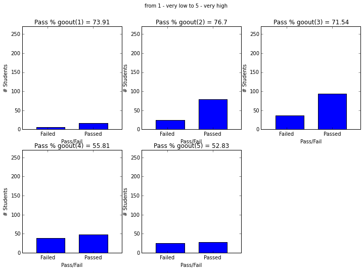
- ‘goout’ going out with friends (numeric: from 1 - very low to 5 - very high)
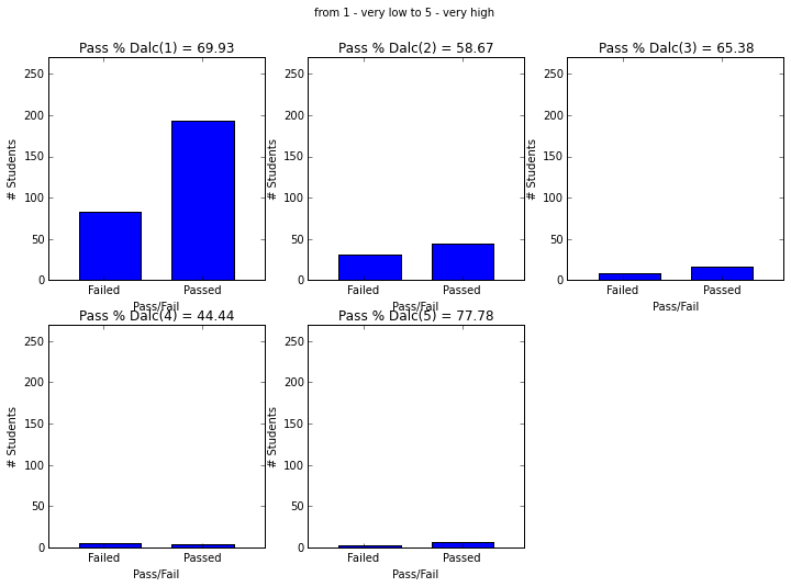
- ‘Dalc’ workday alcohol consumption (numeric: from 1 - very low to 5 - very high)
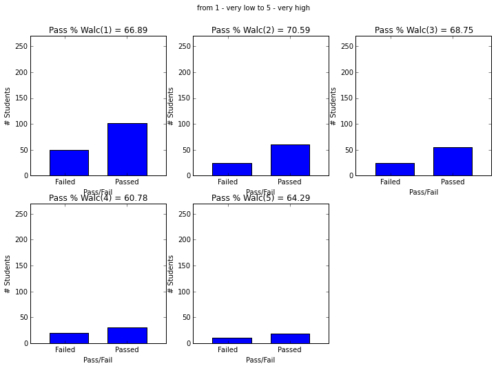
- ‘Walc’ weekend alcohol consumption (numeric: from 1 - very low to 5 - very high)
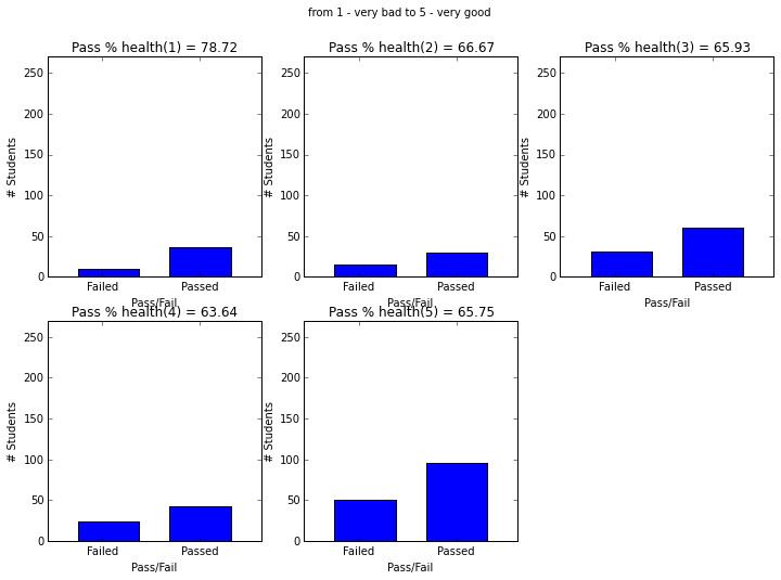
- ‘health’ current health status (numeric: from 1 - very bad to 5 - very good)
- ‘absences’ number of school absences (numeric: from 0 to 93)
- ‘passed’ did the student pass the final exam (binary: yes or no)
The main findings from EDA are,
- Data is collected for 29 factors relating to various socioeconomic, demographic and behavioral indicators of 395 students.
- Of the 395 students, 130 failed and 265 passed. Goal of this project is to identify if a student is at risk for failing based on his/her socioeconomic, demographic and behavioral data.
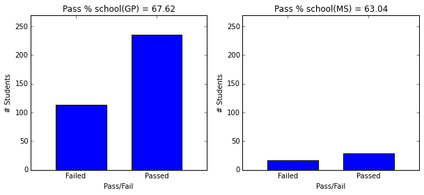
- School GP has much more students than MS, and GP has pass percent of 67.
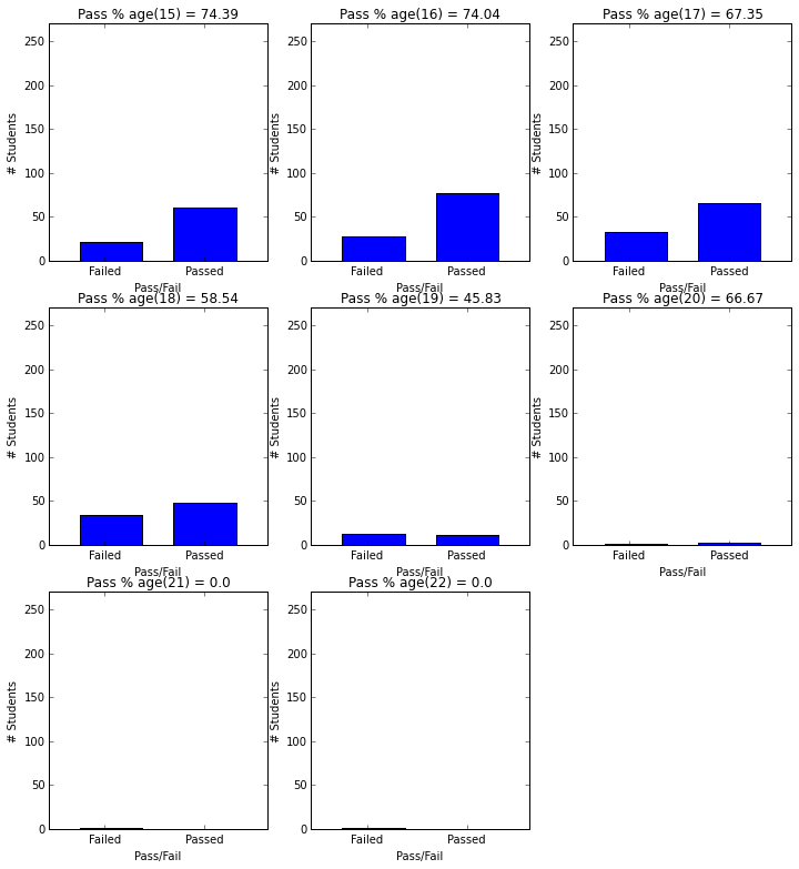
- Students younger than 16 have 74% pass rate, whereas studetns above 21 have 0% pass rate.
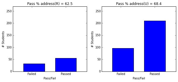
- Students in urban areas (68.5) have higher pass rate than rural (62.5)
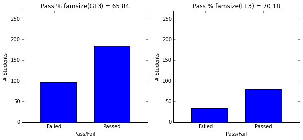
- Smaller families have higher pass rate (70.18) than larger families (65.84).
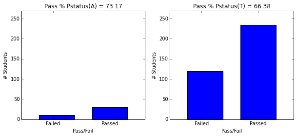
- Students whose parents are apart seem to higher graduation rate (73.2 vs 66.4) however, this may be skewed because to significantly more students’ parents are together
- More mother’s and father’s education is correlated with higher graduation rate.
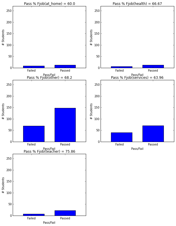
- Mothers with at-home or other jobs have kids with lower pass rates.
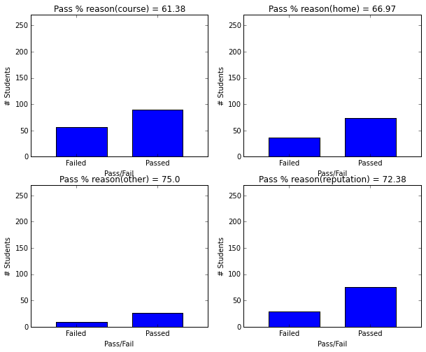
- Student who joined school due to reputation have higher graduation rate.
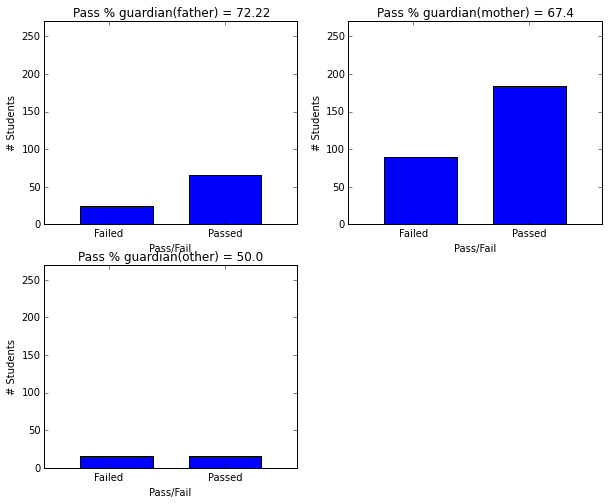
- Students with father as guardian have higher graduation rates (72.22).
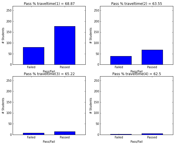
- Students with travel time less than 1 hour have higher pass rate (69) than other students (63)
- Students studying 3 hours or more have more than 74% passing rate.
- Students with fewer failures in past have higher passing rates.
- Students with school and family support have higher passing rate.
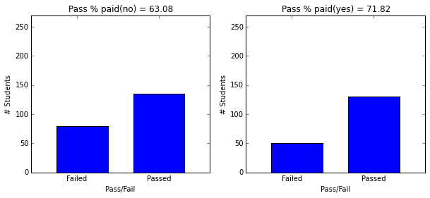
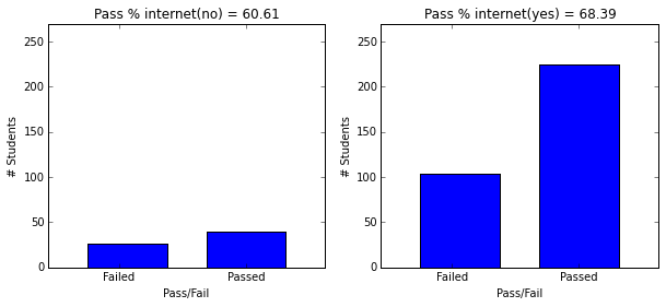
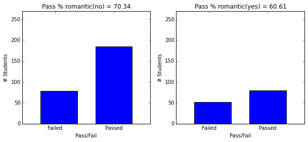
- Students with paid supplemental education, internet access, who go out less and have low daily alcohol consumption have higher passing rate.
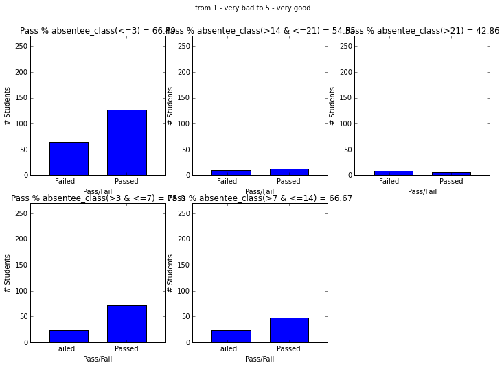
Based on these EDA findings, I grouped age into 4 categories, one below 16, other between 16 and 17, other between 17 and 18, and final above 19. I also grouped absences into fewer categories, less than 3 days, between 3 and 7, 7 and 14, 14 and 21, and more than 21. All the groups include upper value of the interval.
In the next post, I will apply Multiple Correspondence Analysis (MCA), [equivalent of Principal Component Analysis for categorical variables] for dimensionality reduction.
# Import libraries
import numpy as np
import pandas as pd
from time import time
from sklearn.metrics import f1_score
import matplotlib.pyplot as plt
%pylab inline
# Read student data

from sklearn.ensemble import ExtraTreesClassifier
from sklearn.linear_model import LinearRegression
from sklearn.metrics import log_loss, accuracy_score
from sklearn.feature_selection import SelectKBest, f_regression,chi2
Populating the interactive namespace from numpy and matplotlib
# Defining custom functions

def plot_condn(data,condn,title_str):
    # plot by condition
    num_pass = data.passed[data.passed == 'yes'][condn]
    num_fail = data.passed[data.passed == 'no'][condn]
    plt.bar([0.35,.5],[len(num_fail),len(num_pass)],width=.1)
    ax = gca()
    plt.xticks([0.39,.55])
    ax.set_xticklabels(['Failed','Passed'])
    plt.ylim(0,270)
    plt.xlim(0.3,.65)
    plt.ylabel('# Students')
    plt.xlabel('Pass/Fail')

    rat = float(len(num_pass))/float(len(num_pass)+len(num_fail))*100
    plt.title('Pass % ' + title_str +' = '  + str(np.round(rat,2)))
def plot_figures_by_fac(data,fac,n_row_fig,n_col_fig):
    # plot by factor
    fac_unique = np.unique(data[fac])
    i = 1
    for fac_i in fac_unique:
        plt.subplot(n_row_fig,n_col_fig,i)
        condn = (data[fac] == fac_i)
        title_str = fac + '(' + str(fac_i) + ')'
        plot_condn(data,condn,title_str)
        i+=1
def absentee_class(n):
    # Class for absentee.

    class_name = ['<=3','>3 & <=7',
             '>7 & <=14','>14 & <=21','>21']
    limit_class = [0,3,7,14,21,1000]
    abs_class = class_name[0]
    if n!=0:
        lt_n = [i for i in np.arange(0,len(limit_class)) if limit_class[i]<=n-1]
        abs_class = class_name[lt_n[-1]]
    return abs_class
student_data = pd.read_csv("student-data.csv")
print "Student data read successfully!"

student_data['absentee_class'] = student_data.apply(lambda row: absentee_class(row['absences']), axis=1)
student_data = student_data.drop('absences',axis=1)
student_data.columns
target = student_data['passed']
features = student_data.drop('passed',axis=1)
print 'column names', features.columns
print 'number of features', len(features.columns)-1
Student data read successfully!
column names Index([u'school', u'sex', u'age', u'address', u'famsize', u'Pstatus', u'Medu',
       u'Fedu', u'Mjob', u'Fjob', u'reason', u'guardian', u'traveltime',
       u'studytime', u'failures', u'schoolsup', u'famsup', u'paid',
       u'activities', u'nursery', u'higher', u'internet', u'romantic',
       u'famrel', u'freetime', u'goout', u'Dalc', u'Walc', u'health',
       u'absentee_class'],
      dtype='object')
number of features 29
student_data.head()
| school | sex | age | address | famsize | Pstatus | Medu | Fedu | Mjob | Fjob | ... | internet | romantic | famrel | freetime | goout | Dalc | Walc | health | passed | absentee_class | |
|---|---|---|---|---|---|---|---|---|---|---|---|---|---|---|---|---|---|---|---|---|---|
| 0 | GP | F | 18 | U | GT3 | A | 4 | 4 | at_home | teacher | ... | no | no | 4 | 3 | 4 | 1 | 1 | 3 | no | >3 & <=7 |
| 1 | GP | F | 17 | U | GT3 | T | 1 | 1 | at_home | other | ... | yes | no | 5 | 3 | 3 | 1 | 1 | 3 | no | >3 & <=7 |
| 2 | GP | F | 15 | U | LE3 | T | 1 | 1 | at_home | other | ... | yes | no | 4 | 3 | 2 | 2 | 3 | 3 | yes | >7 & <=14 |
| 3 | GP | F | 15 | U | GT3 | T | 4 | 2 | health | services | ... | yes | yes | 3 | 2 | 2 | 1 | 1 | 5 | yes | <=3 |
| 4 | GP | F | 16 | U | GT3 | T | 3 | 3 | other | other | ... | no | no | 4 | 3 | 2 | 1 | 2 | 5 | yes | >3 & <=7 |
5 rows × 31 columns
n_passed = student_data.passed[student_data.passed=='yes'].count()
n_failed = student_data.passed[student_data.passed=='no'].count()
rat_PF = float(n_passed)/float(n_passed+n_failed)*100

print 'Number of students passed is %d and number of failed is %d.' %(n_passed,n_failed)
print 'Current pass percentage is %.2f' %(rat_PF)
Number of students passed is 265 and number of failed is 130.
Current pass percentage is 67.09
n_passed = student_data.passed[(student_data.passed=='yes') & (student_data.sex == 'F')].count()
n_failed = student_data.passed[(student_data.passed=='no') & (student_data.sex == 'F')].count()
rat_PF = float(n_passed)/float(n_passed+n_failed)*100

print 'Number of students passed is %d and number of failed is %d.' %(n_passed,n_failed)
print 'Current pass percentage is %.2f' %(rat_PF)
Number of students passed is 133 and number of failed is 75.
Current pass percentage is 63.94
plt.figure(figsize=(10,4))
plot_figures_by_fac(student_data,'school',1,2)
plt.figure(figsize=(12,13))
plot_figures_by_fac(student_data,'age',3,3)
plt.figure(figsize=(10,4))
plot_figures_by_fac(student_data,'address',1,2)
plt.figure(figsize=(10,4))
plot_figures_by_fac(student_data,'famsize',1,2)
plt.figure(figsize=(10,4))
plot_figures_by_fac(student_data,'Pstatus',1,2)
plt.figure(figsize=(10,13))
plt.suptitle('(0 - none, \n 1 - primary education (4th grade),\n 2- 5th to 9th grade, \n 3 - secondary education or \n 4 -higher education)')
plot_figures_by_fac(student_data,'Medu',3,2)
plt.figure(figsize=(10,13))
plt.suptitle('(0 - none, \n 1 - primary education (4th grade),\n 2- 5th to 9th grade, \n 3 - secondary education or \n 4 -higher education)')
plot_figures_by_fac(student_data,'Fedu',3,2)
plt.figure(figsize=(10,13))
plot_figures_by_fac(student_data,'Mjob',3,2)
plt.figure(figsize=(10,13))
plot_figures_by_fac(student_data,'Fjob',3,2)
plt.figure(figsize=(10,8))
plot_figures_by_fac(student_data,'reason',2,2)
plt.figure(figsize=(10,8))
plot_figures_by_fac(student_data,'guardian',2,2)
plt.figure(figsize=(10,8))
plot_figures_by_fac(student_data,'traveltime',2,2)
plt.figure(figsize=(10,8))
plot_figures_by_fac(student_data,'studytime',2,2)
plt.figure(figsize=(10,8))
plot_figures_by_fac(student_data,'failures',2,2)
plt.figure(figsize=(10,4))
plot_figures_by_fac(student_data,'schoolsup',1,2)
plt.figure(figsize=(10,4))
plot_figures_by_fac(student_data,'famsup',1,2)
plt.figure(figsize=(10,4))
plot_figures_by_fac(student_data,'paid',1,2)
plt.figure(figsize=(10,4))
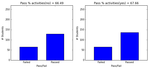
plot_figures_by_fac(student_data,'activities',1,2)
plt.figure(figsize=(10,4))
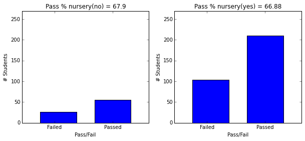
plot_figures_by_fac(student_data,'nursery',1,2)
plt.figure(figsize=(10,4))
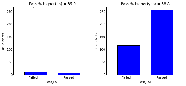
plot_figures_by_fac(student_data,'higher',1,2)
plt.figure(figsize=(10,4))
plot_figures_by_fac(student_data,'internet',1,2)
plt.figure(figsize=(10,4))
plot_figures_by_fac(student_data,'romantic',1,2)
plt.figure(figsize=(12,8))
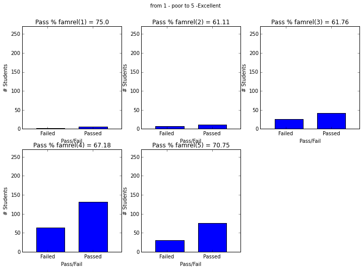
plot_figures_by_fac(student_data,'famrel',2,3)
plt.suptitle('from 1 - poor to 5 -Excellent')
plt.figure(figsize=(12,8))
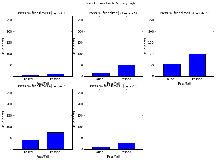
plot_figures_by_fac(student_data,'freetime',2,3)
plt.suptitle('from 1 - very low to 5 - very high')
plt.figure(figsize=(12,8))
plot_figures_by_fac(student_data,'goout',2,3)
plt.suptitle('from 1 - very low to 5 - very high')
plt.figure(figsize=(12,8))
plot_figures_by_fac(student_data,'Dalc',2,3)
plt.suptitle('from 1 - very low to 5 - very high')
plt.figure(figsize=(12,8))
plot_figures_by_fac(student_data,'Walc',2,3)
plt.suptitle('from 1 - very low to 5 - very high')
plt.figure(figsize=(12,8))
plot_figures_by_fac(student_data,'Dalc',2,3)
plt.suptitle('from 1 - very low to 5 - very high')

plt.figure(figsize=(12,8))
plot_figures_by_fac(student_data,'health',2,3)
plt.suptitle('from 1 - very bad to 5 - very good')
plt.figure(figsize=(12,8))
plot_figures_by_fac(student_data,'absentee_class',2,3)
plt.suptitle('from 1 - very bad to 5 - very good')
Additional links - Multiple Correpondance Analysis https://www.utdallas.edu/~herve/Abdi-MCA2007-pretty.pdf - https://github.com/esafak/mca