Multiple Correspondance Analysis (MCA) - Introduction
1. Motivation and overview
Principal component analysis (PCA) is a statistical procedure that uses an orthogonal transformation to convert a set of observations of possibly correlated variables into a set of values of linearly uncorrelated variables called principal components (from Wikipedia). However, PCA assumes that the data is composed of continuous values and contains no categorical variables. It is not possible to apply PCA techniques for dimensionality reduction when the data is composed of categorical variables. Luckily there exists Multiple Correspondance Analysis (MCA), a PCA-like technique developed for categorical data. MCA has been successfully applied for clustering in genomic data or population surveys.
MCA is developed for categorical variables that take values of either 0 or 1. A categorical variable is binarized in cases where it can take more than 2 values. For example, a categorical variable that varies between [1,2,3] can be categorized such that 1 becomes [1,0,0], 2 becomes [0,1,0] and 3 becomes [0,0,1]. The matrix consisiting of data transformed using this process is refered as indicator matrix. MCA is obtained by applying a standard correspondence analysis on this indicator matrix. The result is a linear combination of rows (also referred as factors or factor scores) that best describe the data. As several variables that represent the same quantity are introduced, the variance explained by the components is severely underestimated. Benzécri and then Greenacre proposed corrections to better estimate the explained variances.
In this post I will first explain how MCA can be used to classify wine from two oak barrels based on scoring of multiple wine experts. Next I will present a brief tutorial on using the mca package. First data is downloaded from github repository of the MCA project (link: http://tinyurl.com/hzzswb7). Data source, research article and link to MCA package are included in the acknowledgement section.
Important: ‘pip install mca’ downloads an older version of MCA. The code presented here will not work on the older version. Newer version can be obtained from the github site for the project.
2. Applying MCA to wine data
The wine data consists of ratings from 3 experts on wine aged in 2 distinct barrels. The wine is rated on scales that correspond to fruity, vanillin, coffee, roast and buttery characteristics. Furthermore, not all experts scores the same characteristics of wine. Further, one expert rated woody characteristic on a binary scale of yes/no while other rated it as ordinal quantities ranging from 1 to 3. Due to inconsistencies in how experts rated the wine and differences in characteristics they rated, the task of identifying underlying patterns in this data is very difficult. Further, we wish to predict which barrel a wine came from based on experts’ scores. This is presented in the last row of the table. In case where the experts didnt provide any input, equal score of 0.5 was assigned to all the categorical variables.
MCA however is well suited for such applications. This post explores how MCA can be applied to understand effect of barrel, and how well do experts’ ratings agree with one another.
First the necessary packages are loaded.
import pandas as pd
import numpy as np
from scipy.linalg import diagsvd
%matplotlib inline
import matplotlib.pyplot as plt


import functools
def Matrix_mult(*args):
    """An internal method to multiply matrices."""
    return functools.reduce(np.dot, args)

np.set_printoptions(formatter={'float': '{: 0.4f}'.format})
pd.set_option('display.precision', 5)
pd.set_option('display.max_columns', 25)
Reading wine data
data = pd.read_table('burgundies.csv',
                     sep=',', skiprows=1, index_col=0, header=0)
X = data.drop('oak_type', axis=1)
j_sup = data.oak_type
i_sup = np.array([0, 1, 0, 1, 0, .5, .5, 1, 0, 1, 0, 0, 1, 0, .5, .5, 1, 0, .5, .5, 0, 1])
ncols = 10

X.shape, j_sup.shape, i_sup.shape
src_index = (['Expert 1'] * 7 + ['Expert 2'] * 9 + ['Expert 3'] * 6)
var_index = (['fruity'] * 2 + ['woody'] * 3 + ['coffee'] * 2 + ['fruity'] * 2
             + ['roasted'] * 2 + ['vanillin'] * 3 + ['woody'] * 2 + ['fruity'] * 2
             + ['butter'] * 2 + ['woody'] * 2)
yn = ['y','n']; rg = ['1', '2', '3']; val_index = yn + rg + yn*3 + rg + yn*4
col_index = pd.MultiIndex.from_arrays([src_index, var_index, val_index],
                                      names=['source', 'variable', 'value'])

table1 = pd.DataFrame(data=X.values, index=X.index, columns=col_index)
table1.loc['W?'] = i_sup
table1['','Oak Type',''] = j_sup

table1
| source | Expert 1 | Expert 2 | Expert 3 | ||||||||||||||||||||
|---|---|---|---|---|---|---|---|---|---|---|---|---|---|---|---|---|---|---|---|---|---|---|---|
| variable | fruity | woody | coffee | fruity | roasted | vanillin | woody | fruity | butter | woody | Oak Type | ||||||||||||
| value | y | n | 1 | 2 | 3 | y | n | y | n | y | n | 1 | 2 | 3 | y | n | y | n | y | n | y | n | |
| Wine | |||||||||||||||||||||||
| W1 | 1 | 0 | 0 | 0 | 1 | 0.0 | 1.0 | 1 | 0 | 0 | 1 | 0 | 0 | 1 | 0.0 | 1.0 | 0 | 1 | 0.0 | 1.0 | 0 | 1 | 1 |
| W2 | 0 | 1 | 0 | 1 | 0 | 1.0 | 0.0 | 0 | 1 | 1 | 0 | 0 | 1 | 0 | 1.0 | 0.0 | 0 | 1 | 1.0 | 0.0 | 1 | 0 | 2 |
| W3 | 0 | 1 | 1 | 0 | 0 | 1.0 | 0.0 | 0 | 1 | 1 | 0 | 1 | 0 | 0 | 1.0 | 0.0 | 0 | 1 | 1.0 | 0.0 | 1 | 0 | 2 |
| W4 | 0 | 1 | 1 | 0 | 0 | 1.0 | 0.0 | 0 | 1 | 1 | 0 | 1 | 0 | 0 | 1.0 | 0.0 | 1 | 0 | 1.0 | 0.0 | 1 | 0 | 2 |
| W5 | 1 | 0 | 0 | 0 | 1 | 0.0 | 1.0 | 1 | 0 | 0 | 1 | 0 | 0 | 1 | 0.0 | 1.0 | 1 | 0 | 0.0 | 1.0 | 0 | 1 | 1 |
| W6 | 1 | 0 | 0 | 1 | 0 | 0.0 | 1.0 | 1 | 0 | 0 | 1 | 0 | 1 | 0 | 0.0 | 1.0 | 1 | 0 | 0.0 | 1.0 | 0 | 1 | 1 |
| W? | 0 | 1 | 0 | 1 | 0 | 0.5 | 0.5 | 1 | 0 | 1 | 0 | 0 | 1 | 0 | 0.5 | 0.5 | 1 | 0 | 0.5 | 0.5 | 0 | 1 | NaN |
In table above, the expert 1 rated wine from 1 to 3 for fruitiness where as expert 3 rated this as yes or no. These responses were converted to either 0 or 1 corresponding to each response from the rater. Note that the responses are not uncorrelated. For example, expert 1 rated wine 1 as fruity on a yes/no scale, therefore, if the first column is 1, the next has to be 0. The matrix above is also referred as the indicator matrix. The steps for applying MCA are as follows, 1. Normalize data by dividing by the total of all entries. Note that in the case above, all the rows add up to N, where N is the number of new independent variables formed. 2. Get 2 vectors corresponding to the sum of rows and colums. The row sums are proportional to probability of a wine having a score corresponding to the categorical variables. 3. Compute residual matrix by subtracting the expected indicator matrix (outer product of rows and columns sums computed in step 2). 3. Apply SVD to the residual matrix to compute left- (row) and right- (column) eigenvectors. 4. Choose number of dimensions. This is usually done based on explained variance ratios, however, it is important to apply corrections because the all the categorical variables are not actually uncorrelated.
PS: Percentage of variance explained by an eigen vector is also referred as its inertia.
Normalize
# Normalize
X_values = table1.values[0:6,0:22]
N_all = np.sum(X_values)
Z = X_values/N_all
Compute row and column sums
# Compute row and column sums
Sum_r = np.sum(Z,axis=1)
Sum_c = np.sum(Z,axis=0)

X_values.shape, Sum_r.shape, Sum_c.shape, N_all
Compute residual
# Compute residual
Z_expected = np.outer(Sum_r, Sum_c)
Z_residual = Z - Z_expected

# Scale residual by the square root of column and row sums.
#Note we are computing SVD on residual matrix, not the analogous covariance matrix,
# Therefore, we are dividing by square root of Sums.
D_r = np.diag(Sum_r)
D_c = np.diag(Sum_c)

D_r_sqrt_mi = np.sqrt(np.diag(Sum_r**-1))
D_c_sqrt_mi = np.sqrt(np.diag(Sum_c**-1))

Z_residual.shape, Z.shape, D_r_sqrt_mi.shape,D_c_sqrt_mi.shape
MCA matrix and SVD calculations
MCA_mat = Matrix_mult(D_r_sqrt_mi,Z_residual,D_c_sqrt_mi)
## Apply SVD.
## IN np implementation, MCA_mat = P*S*Q, not P*S*Q'
P,S,Q = np.linalg.svd(MCA_mat)
P.shape,S.shape,Q.shape
# Verify if MCA_mat = P*S*Q,
S_d = diagsvd(S, 6, 22)
sum_mca = np.sum((Matrix_mult(P,S_d,Q)-MCA_mat)**2)
print 'Difference between SVD and the MCA matrix is %0.2f' % sum_mca
Difference between SVD and the MCA matrix is 0.00
Compute factor space, or row and column eigen space
# Compute factor space, or row and column eigen space
F = Matrix_mult(D_r_sqrt_mi,P,S_d) ## Column Space, contains linear combinations of columns
G = Matrix_mult(D_c_sqrt_mi,Q.T,S_d.T) ## Row space, contains linear combinations of rows

F.shape, G.shape
The $S^2$ represents the eigen values (or inertia) for the corresponding factors. Therefore, eigenvalues normalized by the sum of eigen vectors represent the percentage contribution of individual eigen vectors.
Eigen value correction to better estimate contributions of individual eigen vectors.
Lam = S**2
Expl_var = Lam/np.sum(Lam)

print 'Eigen values are ', Lam
print 'Explained variance of eigen vectors are ', Expl_var
Eigen values are  [ 0.8532  0.2000  0.1151  0.0317  0.0000  0.0000]
Explained variance of eigen vectors are  [ 0.7110  0.1667  0.0959  0.0264  0.0000  0.0000]
The first 2 components explain more than 87% of the variance in the data. However, these values are underestimated because the underlying categorical variables are not truly independent. In fact, it can be shown that all the factors with an eigenvalue less or equal to 1/K simply code the additional dimensions. K is the number of true independent measures. In our case, K = 10. Two corrections formulas are used to correct, the first one is due to Benzécri (1979), the second one to Greenacre (1993).
Benzécri correction
Benzécri identifies the fact that the eigen values below 1/K represent variations due to addition of additional variables. Therefore, in Benzécri correction, the values below 1/K are dropped and the remaining eigen values are scaled by a factor of K/(K-1). After performing this calculation, the percentage of variance explained by the first component went up to 98.2%. However, Benzécri correction tends to give an optimistic estimate of variance. Greenacre proposed another correction.
K = 10
E = np.array([(K/(K-1.)*(lm - 1./K))**2 if lm > 1./K else 0 for lm in S**2])
Expl_var_bn = E/np.sum(E)
print 'Eigen vectors after Benzécri correction are ' , E
print 'Explained variance of eigen vectors after Benzécri correction are ' , Expl_var_bn
Eigen vectors after Benzécri correction are  [ 0.7004  0.0123  0.0003  0.0000  0.0000  0.0000]
Explained variance of eigen vectors after Benzécri correction are  [ 0.9823  0.0173  0.0004  0.0000  0.0000  0.0000]
Greenacre correction
Greenacre proposed a different normalization scheme instead of dividing the eigen vectors by the sum of eigen values. This method gives slightly more conservative estimate of contribution of eigen vectors.
J = 22.
green_norm = (K / (K - 1.) * (np.sum(S**4)
                                 - (J - K) / K**2.))
# J is the number of categorical variables. 22 in our case.

print 'Explained variance of eigen vectors after Greenacre correction are ' , E/green_norm
Explained variance of eigen vectors after Greenacre correction are [ 0.9519 0.0168 0.0004 0.0000 0.0000 0.0000]
#####
data = {'Iλ': pd.Series(Lam),
        'τI': pd.Series(Expl_var),
        'Zλ': pd.Series(E),
        'τZ': pd.Series(Expl_var_bn),
        'cλ': pd.Series(E),
        'τc': pd.Series(E/green_norm),
        }
columns = ['Iλ', 'τI', 'Zλ', 'τZ', 'cλ', 'τc']
table2 = pd.DataFrame(data=data, columns=columns).fillna(0)
table2.index += 1
table2.loc['Σ'] = table2.sum()
table2.index.name = 'Factor'
np.round(table2.astype(float), 4)
| Iλ | τI | Zλ | τZ | cλ | τc | |
|---|---|---|---|---|---|---|
| Factor | ||||||
| 1 | 0.8532 | 0.7110 | 0.7004 | 0.9823 | 0.7004 | 0.9519 |
| 2 | 0.2000 | 0.1667 | 0.0123 | 0.0173 | 0.0123 | 0.0168 |
| 3 | 0.1151 | 0.0959 | 0.0003 | 0.0004 | 0.0003 | 0.0004 |
| 4 | 0.0317 | 0.0264 | 0.0000 | 0.0000 | 0.0000 | 0.0000 |
| 5 | 0.0000 | 0.0000 | 0.0000 | 0.0000 | 0.0000 | 0.0000 |
| 6 | 0.0000 | 0.0000 | 0.0000 | 0.0000 | 0.0000 | 0.0000 |
| Σ | 1.2000 | 1.0000 | 0.7130 | 1.0000 | 0.7130 | 0.9691 |
Squared cosine distance and contributions
Squared cosine distance between factor $l$ (analogous to principal component) and column $j$ is given by $g^2{j,l}/d{c,j}^2$, and between factor $l$ (analogous to principal component) and row $i$ is given by $f^2{i,l}/d{r,i}^2$.
Similarly, contributions of row $i$ to factor $l$ and of coloumn $j$ to factor $l$ are given by, $f^2{i,l}/\lambda{l}^2$ and $g^2{j,l}/\lambda{l}^2$ respictively.
d_c = np.linalg.norm(G, axis=1)**2 # Same as np.diag(G*G.T)
d_r = np.linalg.norm(F, axis=1)**2 # Same as np.diag(F*F.T)
# Cosine distance between factors and first 4 components
CosDist_c = np.apply_along_axis(lambda x: x/d_c, 0, G[:, :4]**2)
# Cosine distance between factors and first 4 components
CosDist_r = np.apply_along_axis(lambda x: x/d_r, 0, F[:, :4]**2)
# Cosine distance between factors and first 4 components
Cont_c = np.apply_along_axis(lambda x: x, 0, G[:, :4]**2)
# Cosine distance between factors and first 4 components
Cont_r = np.apply_along_axis(lambda x: x, 0, F[:, :4]**2)
Projecting data from feature space to reduced factor space.
A vector from original feature space can be projected on the reduced by taking inner product by individual features and scaling it by appropriately. In the current example, the projections are given by,
## Projecting vectors onto factor space.
X_pjn = []
for i in np.arange(0,6):
    X_pjn.append(np.dot(X.iloc[i],G[:,:4])/S[:4]/10)

X_pjn = np.asarray(X_pjn)

## The projection can also be computed using vectorized form,
X_pjn = Matrix_mult(X.values,G[:,:4])/S[:4]/10
X_i = -Matrix_mult(i_sup,G[:,:4])/S[:4]/10
fs, cos = 'Factor score','Squared cosines'
table3 = pd.DataFrame(columns=['W1','W2','W3','W4','W5','W6'], index=pd.MultiIndex
                      .from_product([[fs, cos], range(1, 3)]))

#table3.loc[fs,    :] = mca_ind.fs_r(N=2).T
#table3.loc[cos,   :] = mca_ind.cos_r(N=2).T
#table3.loc[cont,  :] = mca_ind.cont_r(N=2).T * 1000

fs, cos, cont = 'Factor score','Squared cosines', 'Contributions x 1000'
table3 = pd.DataFrame(columns=X.index, index=pd.MultiIndex.from_product([[fs, cos], range(1, 5)]))

table3.loc[fs,    :] = X_pjn[:,:4].T
table3.loc[cos,   :] = CosDist_r.T

np.round(table3.astype(float), 2)
| Wine | W1 | W2 | W3 | W4 | W5 | W6 | |
|---|---|---|---|---|---|---|---|
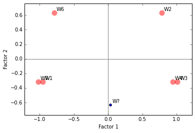
| Factor score | 1 | -0.95 | 0.79 | 1.02 | 0.95 | -1.02 | -0.79 |
| 2 | -0.32 | 0.63 | -0.32 | -0.32 | -0.32 | 0.63 | |
| 3 | 0.43 | 0.39 | 0.10 | -0.43 | -0.10 | -0.39 | |
| 4 | 0.10 | -0.18 | 0.23 | -0.10 | -0.23 | 0.18 | |
| Squared cosines | 1 | 0.75 | 0.52 | 0.86 | 0.75 | 0.86 | 0.52 |
| 2 | 0.08 | 0.33 | 0.08 | 0.08 | 0.08 | 0.33 | |
| 3 | 0.15 | 0.12 | 0.01 | 0.15 | 0.01 | 0.12 | |
| 4 | 0.01 | 0.03 | 0.04 | 0.01 | 0.04 | 0.03 |
From factor projections, it is clear that the values of first factor are negative for the barrel 1, and positive for the barrel 2. This is better illustrated in the figure below. The scores for unknown wine is represented by the blue dot. Based on these ratings, its not possible to accurately assign the new wine to either of the two barrels.
points = table3.loc[fs].values
labels = table3.columns.values

plt.figure()
plt.margins(0.1)
plt.axhline(0, color='gray')
plt.axvline(0, color='gray')
plt.xlabel('Factor 1')
plt.ylabel('Factor 2')
plt.scatter(X_pjn[:,0],X_pjn[:,1], marker='o',s=120, color='r', alpha=.5, linewidths=0)
i = 0
for label in X.index:
    x = X_pjn[i,0]
    y = X_pjn[i,1]
    plt.annotate(label, xy=(x, y), xytext=(x + .03, y + .03))
    i +=1
plt.scatter(X_i[0],X_i[1])
plt.annotate('W?', xy=(X_i[0],X_i[1]), xytext=(X_i[0] + .03, X_i[1] + .03))

plt.show()
3. Quick tutorial on MCA package.
Now we will apply the MCA package in python to perform the same calculations.
from mca import *

data = pd.read_table('burgundies.csv',
                     sep=',', skiprows=1, index_col=0, header=0)
X = data.drop('oak_type', axis=1)
j_sup = data.oak_type
i_sup = np.array([0, 1, 0, 1, 0, .5, .5, 1, 0, 1, 0, 0, 1, 0, .5, .5, 1, 0, .5, .5, 0, 1])
ncols = 10
MCA calculations are implemented via MCA object. The default condition applies Benzécri correction for eigen values, therefore, benzecri flag has to be set to false. Below are the list of attributes for the MCA function, - .L Eigen values - .F Factor scores for columns. (components are linear combination of columns) - .G Factor scores for rows. (components are linear combination of rows) - .expl_var Explained variance. - .fs_r Projections onto the factor space, can also be computed by applying fs_r_sup on each of the row elements. - .cos_r Cosine distance between $i^{th}$ vector and $j^{th}$ factor (or row eigen vector) - .cont_r Contribution of individual categorical variable to the factor.
mca_ben = MCA(X, ncols=ncols)
mca_ind = MCA(X, ncols=ncols, benzecri=False)
data = {'Iλ': pd.Series(mca_ind.L),
        'τI': mca_ind.expl_var(greenacre=False, N=4),
        'Zλ': pd.Series(mca_ben.L),
        'τZ': mca_ben.expl_var(greenacre=False, N=4),
        'cλ': pd.Series(mca_ben.L),
        'τc': mca_ind.expl_var(greenacre=True, N=4)}

# 'Indicator Matrix', 'Benzecri Correction', 'Greenacre Correction'
columns = ['Iλ', 'τI', 'Zλ', 'τZ', 'cλ', 'τc']
table2 = pd.DataFrame(data=data, columns=columns).fillna(0)
table2.index += 1
table2.loc['Σ'] = table2.sum()
table2.index.name = 'Factor'

table2
| Iλ | τI | Zλ | τZ | cλ | τc | |
|---|---|---|---|---|---|---|
| Factor | ||||||
| 1 | 0.8532 | 0.7110 | 0.7004 | 0.9823 | 0.7004 | 0.9519 |
| 2 | 0.2000 | 0.1667 | 0.0123 | 0.0173 | 0.0123 | 0.0168 |
| 3 | 0.1151 | 0.0959 | 0.0003 | 0.0004 | 0.0003 | 0.0004 |
| 4 | 0.0317 | 0.0264 | 0.0000 | 0.0000 | 0.0000 | 0.0000 |
| Σ | 1.2000 | 1.0000 | 0.7130 | 1.0000 | 0.7130 | 0.9691 |
Next we will use functions in MCA to compute the projections onto important factors, cosine distance and contributions of individual terms to the factors.
fs, cos, cont = 'Factor score','Squared cosines', 'Contributions x 1000'
table3 = pd.DataFrame(columns=X.index, index=pd.MultiIndex
                      .from_product([[fs, cos, cont], range(1, 3)]))

table3.loc[fs,    :] = mca_ben.fs_r(N=2).T
table3.loc[cos,   :] = mca_ben.cos_r(N=2).T
table3.loc[cont,  :] = mca_ben.cont_r(N=2).T * 1000
table3.loc[fs, 'W?'] = mca_ben.fs_r_sup(pd.DataFrame([i_sup]), N=2)[0]

np.round(table3.astype(float), 2)
| Wine | W1 | W2 | W3 | W4 | W5 | W6 | W? | |
|---|---|---|---|---|---|---|---|---|
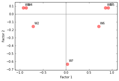
| Factor score | 1 | 0.86 | -0.71 | -0.92 | -0.86 | 0.92 | 0.71 | 0.03 |
| 2 | 0.08 | -0.16 | 0.08 | 0.08 | 0.08 | -0.16 | -0.63 | |
| Squared cosines | 1 | 0.99 | 0.95 | 0.99 | 0.99 | 0.99 | 0.95 | NaN |
| 2 | 0.01 | 0.05 | 0.01 | 0.01 | 0.01 | 0.05 | NaN | |
| Contributions x 1000 | 1 | 176.68 | 120.99 | 202.33 | 176.68 | 202.33 | 120.99 | NaN |
| 2 | 83.33 | 333.33 | 83.33 | 83.33 | 83.33 | 333.33 | NaN |
%matplotlib inline
import matplotlib.pyplot as plt

points = table3.loc[fs].values
labels = table3.columns.values

plt.figure()
plt.margins(0.1)
plt.axhline(0, color='gray')
plt.axvline(0, color='gray')
plt.xlabel('Factor 1')
plt.ylabel('Factor 2')
plt.scatter(*points, s=120, marker='o', c='r', alpha=.5, linewidths=0)
for label, x, y in zip(labels, *points):
    plt.annotate(label, xy=(x, y), xytext=(x + .03, y + .03))
plt.show()
4. Conclusion
In this post, multiple correspondance analysis, a principal component analysis like technique for categorical data is presented. First the method of MCA was presented using python code, then the MCA package was introduced. In the next post I will apply this technique to a more complex problem of identifying at risk students from demographic and behavioral data.
5. Acknowledgements
- Source of Data https://github.com/esafak/mca/tree/master/data
- MCA github https://github.com/esafak/mca
- Link to the paper https://www.utdallas.edu/~herve/Abdi-MCA2007-pretty.pdf Abdi, H., & Valentin, D. (2007). Multiple correspondence analysis. In N.J. Salkind (Ed.): Encyclopedia of Measurement and Statistics. Thousand Oaks (CA): Sage. pp. 651-657.